Differential Drive Robot Odometry Simulation In Python

Understanding and Simulating Differential Drive in Python

When I started building robots, they were super simple. Just motors and wires slapped together on a chassis. I could make them move around, but there was no proper control. The robot had no idea where it was. If I told the robot to move forward 1 meter, it would spin its wheels and think it did the job. But in reality? It might’ve gone 10 cm… or 10 meters. It had no sense of position. It didn’t know where it started or where it ended up.

This is where Odometry comes in. Wheel Odometry uses internal robot sensors to determine the position and orientation of the robot. It is simple and easy to implement for differential drive robots (the classic two-wheeled robot). By doing some maths, we can make our dumb robot very smart. In this article, we’ll do simple math, use some real-world intuition, and solve the problem. We’ll also do a Python simulation that follows a square path using distance-based odometry calculations.

Note: This post builds on the general concepts of odometry. If you’re brand new to the term, check out my other post: What is odometry?

1. What Is Wheel Odometry

Imagine you’re blindfolded and walking straight. You count your steps and measure how long each one is. That’s basically what a robot does with wheel odometry. It measures how much each wheel turns and uses that information to guess how far it’s moved and in what direction.

At the heart of any differential drive robot is a simple but powerful concept: two wheels working together to move the robot forward or rotate it. The two wheels act like legs that provide both forward movement and turning, depending on how they spin.

Each wheel on the robot has its own motor that drives it, and each wheel can rotate at different speeds. The main idea here is:

• When both wheels move at the same speed, the robot moves in a straight line. No turns, just pure forward movement.
• When the wheels move at different speeds, the robot starts to turn. It’s almost like you’re trying to spin around in place by making one leg go faster than the other.

Let’s break that down:

• The left wheel moves a certain distance, say dL.
• The right wheel moves a different distance, say dR.

The robot’s ability to move in a straight line or turn is based on how much each wheel has moved. If both wheels move the same amount, the robot moves straight ahead. But if one wheel moves more than the other, it causes the robot to rotate, following an arc.

This is where the “brain” of the robot comes in: the controller or the odometry algorithm that calculates how the robot is positioned and how it moves based on the wheel data. This information is processed to update the robot’s position and heading, allowing it to track its movement over time.

2. Maths Behind Odometry

Odometry is simple to implement. We just need some high school maths, some sensor data, and we are good :). Like in every maths problems, we will make some assumptions.

1. The robot has two wheels, left and right.
2. Each wheel has a sensor to calculate how distance it has moved.
3. There is no slippage, and sensor data is free of noise.

These assumptions will make calculations easy, but in real life, there will be slippage on the wheels, and sensor data will be noisy. Our goal today is to learn the math behind odometry. We will deal with all the noise when we actually implement this in a real robot, which we will do in another blog. We will implement odometry using the kinematics equations. We will derive and go into details in another blog, for some smart people have already cooked these equations for us, we just need to take them out of the refrigerator, microwave and enjoy.

Declare Some Variables

• dL: Distance traveled by the left wheel.
• dR: Distance traveled by the right wheel.
• L: Distance between the two wheels (the wheelbase).
• θ: Theta is the current orientation (heading) of the robot, typically in radians.
• x, y: The robot’s current position on a 2D plane.

Case 1: Moving Straight

If both wheels travel the same distance, say dL = dR = d, the robot moves forward in a straight line.

The average distance the robot moves forward is the same for both wheels, so we don’t need to calculate any difference:

The robot moves straight in the direction it’s already facing. The orientation doesn’t change, and the robot simply moves forward by the distance d.

Case 2: Turning

If the wheels move different distances, the robot turns in place. This is where the real math comes in.

To understand how much the robot turns, we use this formula:

• dθ: The change in orientation (angle turned by the robot).
• dR: Distance traveled by the right wheel.
• dL: Distance traveled by the left wheel.
• L: Distance between the two wheels (wheelbase).

This equation calculates the change in orientation (how much the robot turns) based on the difference in the distances traveled by the left and right wheels.

• If dR > dL, the robot turns to the left.
• If dL > dR, the robot turns to the right.

Now, we can calculate the robot’s new position after it has moved:

1. Change in orientation (dθ) tells us how much the robot’s heading has changed.
2. Average forward movement (dCenter) tells us how far the robot has moved forward (along an arc, in the case of turning).

The Final Robot Position

Once we know the change in orientation and forward movement, we can update the robot’s position. Imagine the robot is standing at a point on a graph, like on your math notebook, at point (x, y). Now it wants to move forward in the direction it’s facing. The robot might be facing at any angle, like 30° or 45°. So, how do we know how much it has moved in the (x, y) direction? This is where cosine and sine come in.

When a robot moves forward by a small distance d at an angle θ (theta), we break that motion into two parts:

• sin(θ) gives us how much of that motion is in the y-direction (vertical)

• cos(θ) gives us how much of that motion is in the x-direction (horizontal)

The new position (x, y) can be calculated using these equations:

Where:

• x and y are the current position of the robot.
• θ is the current orientation (angle).
• dθ is the change in orientation (calculated from the difference in the wheel distances).
• dCenter is the average distance traveled by both wheels.

These equations work together to update the robot’s position on a 2D plane. In these equations, we are adding the new values (current position and orientation) to the calculated old values of the robot’s motion. Without this, the robot will lose track of its past location and orientation, and the robot wouldn’t know where it is on the map. It will only know how much it has moved for a certain period of time, but it wouldn’t be able to tell its actual positions with respect to the starting point. Adding the new values to the old ones helps solve this problem.

3. Calculating Odometry

Now let’s implement the above equations by using an example. We will test this in Python by passing some parameters to the program, and it will give us the robot position in the form of a graph.

• Assume the left wheel (dL) travels 10 cm, and the right wheel (dR) travels 12 cm.
• The distance between the two wheels (L) is 5 cm.
• The robot’s initial position is (x, y) = (0, 0), and its initial orientation is θ = 0 (facing right).

Step 1: Calculate dθ (change in orientation)

The robot has turned 0.4 radians (about 22.9 degrees).

Step 2: Calculate dCenter (average forward distance)

The robot has moved 11 cm along its path.

Step 3: Calculate the new position (x, y)

Now we use the equations to calculate the new position:

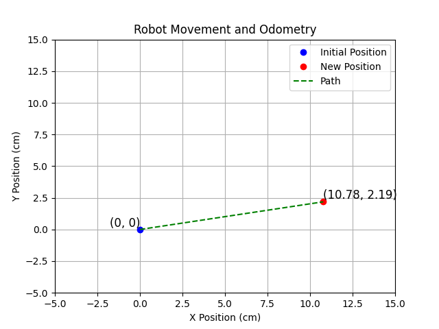
So, after the movement, the robot’s new position is approximately (10.88, 2.19).

Step 4: Update orientation

The new orientation (θ) is:

So, the robot has moved 11 cm and turned 0.4 radians (22.9 degrees), and its new position is (10.88, 2.19) with an orientation of 0.4 radians.

Step 5: Test it in Python.

Let’s Implement this in Python. Run this code in Python you will see the output in the form of a graph, where we will see the old and new position of the robot. You change the parameters of your robot for experimenting.

import math
import matplotlib.pyplot as plt

# Constants
dL = 10  # Distance traveled by left wheel in cm
dR = 12  # Distance traveled by right wheel in cm
L = 5    # Distance between the two wheels (wheelbase) in cm

# Step 1: Calculate change in orientation (dTheta)
dTheta = (dR - dL) / L
print(f"Change in orientation (dTheta): {dTheta:.2f} radians")

# Step 2: Calculate the average forward movement (dCenter)
dCenter = (dL + dR) / 2
print(f"Average forward movement (dCenter): {dCenter:.2f} cm")

# Step 3: Calculate the new position (x, y)
# Initial position (x, y) = (0, 0) and initial orientation = 0
x, y, theta = 0, 0, 0

# Calculate the new position after moving
x_new = x + dCenter * math.cos(theta + dTheta / 2)
y_new = y + dCenter * math.sin(theta + dTheta / 2)
theta_new = theta + dTheta

print(f"New position (x, y): ({x_new:.2f}, {y_new:.2f}) cm")
print(f"New orientation (theta): {theta_new:.2f} radians")

# Plotting the initial and new position of the robot
fig, ax = plt.subplots()

# Initial position (0, 0)
ax.plot(0, 0, 'bo', label="Initial Position")

# New position after movement
ax.plot(x_new, y_new, 'ro', label="New Position")

# Plotting the path (just a line for simplicity)
ax.plot([0, x_new], [0, y_new], 'g--', label="Path")

# Adding labels
ax.text(0, 0, '(0, 0)', fontsize=12, verticalalignment='bottom', horizontalalignment='right')
ax.text(x_new, y_new, f'({x_new:.2f}, {y_new:.2f})', fontsize=12, verticalalignment='bottom')

# Set plot limits and labels
ax.set_xlim(-5, 15)
ax.set_ylim(-5, 15)
ax.set_xlabel("X Position (cm)")
ax.set_ylabel("Y Position (cm)")

# Add title and legend
ax.set_title("Robot Movement and Odometry")
ax.legend()

# Show the plot
plt.grid(True)
plt.show()

1. Initial Setup: The robot starts at the origin (0,0) with an initial orientation of 0 radians (facing straight ahead).
2. Mathematical Calculations:
   • dTheta is the change in orientation, calculated using the difference in the distances traveled by the left and right wheels, divided by the wheelbase.
   • dCenter is the average forward movement, which is simply the average of the distances traveled by both wheels.
   • The robot’s new position and orientation are calculated using the provided equations.
3. Visualization:
   • The code is used matplotlib to plot the initial and new positions of the robot.
   • The path is shown as a green dashed line connecting the initial position to the new position.

4. Simulating a Differential Drive Robot in Python

Now let’s simulate a differential drive robot moving in a square path and visualize its motion using matplotlib. The robot starts at (0,0)(0, 0) facing straight along the positive x-axis. It has parameters like the distance between its wheels (wheelbase) and how far it moves per step (step_size). It asks the user for the size of the square’s side (in centimeters).

• move_forward(distance): Moves the robot forward by calculating its new (x,y)(x, y) position based on its orientation (θ\theta).
• turn_left(angle_rad): Rotates the robot 90 degrees to the left by adjusting its orientation.

This is an example for you to explore. Here you can see the robot move with animations. Please play around with the code for a better understanding.

import math
import matplotlib.pyplot as plt
import matplotlib.animation as animation

# Robot parameters
wheelbase = 5  # Distance between wheels (in cm)
step_size = 1  # Step size (in cm)

# Initial position and orientation of the robot
x, y, theta = 0.0, 0.0, 0.0
poses = [(x, y)]  # Store the robot's path

# User input for square size
square_size = float(input("Enter the size of the square path (in cm): "))

# Function to move the robot forward
def move_forward(distance):
    global x, y, theta
    steps = int(distance / step_size)
    for _ in range(steps):
        dx = step_size * math.cos(theta)
        dy = step_size * math.sin(theta)
        x += dx
        y += dy
        poses.append((x, y))

# Function to turn the robot 90 degrees to the left
def turn_left(angle_rad):
    global theta
    steps = int(abs(angle_rad) / math.radians(5))  # 5° per step
    dtheta = angle_rad / steps
    for _ in range(steps):
        theta += dtheta
        poses.append((x, y))  # Turning in place, position stays the same

# Drive the robot in a square path
for _ in range(4):
    move_forward(square_size)  # Move forward by the size of the square
    turn_left(math.radians(90))  # Turn 90 degrees after each side

# --- Animation Setup ---
fig, ax = plt.subplots()
ax.set_aspect('equal')
margin = square_size * 0.5
ax.set_xlim(-margin, square_size + margin)
ax.set_ylim(-margin, square_size + margin)
line, = ax.plot([], [], 'b-', linewidth=2)
dot, = ax.plot([], [], 'ro', markersize=8)

# Initialize the plot
def init():
    line.set_data([], [])
    dot.set_data([], [])
    return line, dot

# Update the plot for each frame
def update(frame):
    if frame == 0:
        # At the first frame, just plot the initial position
        x_data, y_data = [poses[0][0]], [poses[0][1]]
    else:
        x_data, y_data = zip(*poses[:frame+1])  # Plot all positions up to the current frame
    line.set_data(x_data, y_data)
    dot.set_data([x_data[-1]], [y_data[-1]])  # Make sure these are sequences
    return line, dot

# Set up the animation
ani = animation.FuncAnimation(
    fig, update,
    frames=len(poses),
    init_func=init,
    interval=30,
    blit=True,
    repeat=False
)

plt.title("Robot Following Square Path Using Odometry")
plt.xlabel("X Position (cm)")
plt.ylabel("Y Position (cm)")
plt.grid(True)
plt.show()

1. Robot Parameters:
   • wheelbase = 5: This represents the distance between the two wheels (in centimeters).
   • step_size = 1: This defines how far the robot moves in one step (in centimeters).
2. Initial Position:
   • x, y, theta = 0.0, 0.0, 0.0: The robot starts at the origin (0, 0) facing along the positive x-axis (theta = 0).
3. Square Size:
   • The user is prompted to input the size of the square path in centimeters.
4. Movement Functions:
   • move_forward(distance): This function moves the robot forward a specified distance. It calculates the movement based on the step_size and updates the robot’s position.
   • turn_left(angle_rad): This function turns the robot by a specified angle (in radians). After each turn, the robot’s orientation theta is updated.
5. Driving the Square Path:
   • The robot moves forward for the length of each side of the square (move_forward(square_size)) and then turns 90 degrees (turn_left(math.radians(90))). This process is repeated four times to form a square path.
6. Animation:
   • The robot’s path is displayed using matplotlib With an animation that updates the plot frame by frame.
   • The robot’s position is updated at each step and displayed on the plot. The initial position is marked with a green dot, and the robot’s path is shown with a blue line. The robot’s final position is marked with a red dot.

Running the Program:

1. The program will ask you to input the square size in centimeters.
2. The robot will move along the square path and turn at each corner.
3. You’ll see the robot’s movement animated live.

5. References

• [1] R. Siegwart, I. R. Nourbakhsh, D. Scaramuzza, Introduction to Autonomous Mobile Robots, MIT Press, 2011.
• [2] S. Thrun, W. Burgard, D. Fox, Probabilistic Robotics, MIT Press, 2005.
• [3] Columbia University, “Mobile Robot Kinematics,” [Online]. Available: https://www.cs.columbia.edu/~allen/F17/NOTES/icckinematics.pdf
• [4] Matplotlib Developers, “matplotlib.animation — Matplotlib 3.8.0 documentation,” [Online]. Available: https://matplotlib.org/stable/api/animation_api.html
• [5] National Instruments, “Encoder Basics,” [Online]. Available: https://www.ni.com/en-us/innovations/encoder-basics.html