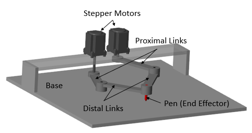
Five Bar Parallel Mechanism Planar Robot Arm

One of the simplest and elegant robot arm designs is the 5R linkage mechanism. The 5R robot arm is a type of parallel manipulator, which sets it apart from the more common serial robots. A serial robot is like your own arm, one joint connected to another, like a chain. Your shoulder connects to your upper arm, then to your elbow, forearm, wrist, and finally your hand. But a parallel robot is different. Instead of having a single chain of joints, it has multiple linkages working together in parallel to control the same end-effector. The 5R or five-bar robot arm uses a mechanical structure to create complex motion using just two motors. In some cases, serial robots cannot provide the necessary performance during operations that require high acceleration and precise motion due to the flexibility of the manipulator; therefore, manipulators with parallel kinematic structure are preferred in such cases. That’s the beauty of parallel linkages—simple input, coordinated output. I have used this concept in some of my projects, like a robot dog leg. This type of mechanism is easy to implement as a robot leg. In this article, I will explain what a five-bar linkage mechanism is and how you can also implement it in your projects using inverse kinematics. Although there are multiple ways we can use this mechanism in this article, we will focus on the five-bar linkage mechanism being used as a parallel SCARA robot arm or 5R Planar robot arm. There are many names for this concept.

1. 5R Parallel Robot Structure

Imagine two separate arms reaching from the base to the same tool, and both arms cooperating to move that tool precisely. In a 5R parallel linkage, there are two chains made of bars or links, and both start from the base and meet at the end-effector. The “5R” name comes from the five revolute or rotational joints in the mechanism. Imagine 5 sticks joined together in a loop using hinges, and you can rotate them at the joints. It forms a closed loop, which means that everything is connected in a way that if one part moves, the whole system adjusts automatically.

Typically, there are two motors placed at the base. These motors drive the first two links, and the rest of the mechanism follows because all the links are mechanically connected. So, when one motor rotates, it doesn’t just move one part—it affects the entire loop. This coordinated motion is what gives the 5R mechanism its precision and strength.

How many ways can a 5R robot arm move move?. In the case of a planar 5R arm (which moves in a flat, 2D plane), we usually get two degrees of freedom, controlled by the two motors. These give us:

• Movement left-right (x-axis)
• Movement forward-backward (y-axis)

2. Advantages of a Parallel Robotic Arm

The 5R robot arm is a smart and efficient design that uses five links and five rotating joints to create fast and accurate motion, mostly within a flat, 2D space. Thanks to its parallel structure, it offers big advantages: it’s quick, precise, and can handle a decent amount of weight for its size.

The 5R linkage robot arm comes with some pretty cool advantages that make it a smart choice for certain tasks. Let me break them down:

1. It’s fast: One big reason for this is where the motors are placed. In a 5R arm, the motors sit right at the base, which doesn’t move. This means all the moving parts—the actual arms and links—can be made light. And lighter parts are easier to move quickly. Less weight = less inertia = faster acceleration and deceleration.
2. It’s accurate: Thanks to its parallel structure, the 5R arm is also really precise. Multiple arms are working together to control the end-effector. This gives the whole system more stiffness and rigidity, which helps reduce wobble or unintended motion. Any small errors in movement tend to balance out across the mechanism, instead of stacking up like they can in a serial robot.
3. It can lift more than you’d expect: For its size and weight, the 5R arm can often handle a decent payload. That’s because the force of whatever it’s lifting is shared across multiple links, rather than all being dumped on a single joint or motor. This load distribution gives the arm a mechanical advantage when it comes to lifting or holding heavier tools or objects.
4. It’s easier to control: The 5R arm, with just two degrees of freedom in the plane, is much simpler to control. You still need some math and control systems, but you won’t be pulling your hair out trying to keep six joints in sync. It’s a great balance of performance and simplicity.
5. It’s energy efficient: Since the motors are fixed at the base and not being lugged around with every movement, the robot uses less energy overall. You don’t have to burn extra power moving heavy motors through space. That makes the whole system more efficient and sometimes even longer-lasting.

3. Applications of the 5R Parallel Robot Arm

The clever linkage design comes with a handful of solid advantages that make it a great fit for many practical applications. Even though the 5R robot arm has some limitations—like working mainly in flat, 2D spaces—it’s surprisingly useful in a variety of real-world tasks, especially where speed and precision are essential. You’ll find it working behind the scenes in factories, animation studios, medical devices, and even toys.

1. Industrial Automation
In factories, 5R robot arms are often used for pick-and-place tasks—moving objects quickly and accurately from one spot to another. They’re also great for assembly lines, especially for small, delicate parts like electronic components. Thanks to their speed, they shine in packaging lines too, sorting and packing items with robotic consistency. Some lightweight machining operations—like drilling or milling on a flat surface—also benefit from the stable, precise motion of 5R arms.

2. Medical & Prosthetic Devices
In healthcare, 5R mechanisms pop up in prosthetics—for example, in ankle-foot systems that mimic natural movement using clever mechanical linkages. They’re also used in haptic feedback devices, which simulate the feeling of touch in VR or remote robotic systems. Some advanced surgical robots use spherical versions of the 5R mechanism to perform super-precise movements in tight spaces during minimally invasive surgeries.

3. Everyday & Educational Tools
Believe it or not, you might’ve seen 5R-like mechanisms in fun gadgets too—like automatic drawing toys (e.g., WeDraw), or even in modified forms inside vehicle steering systems like Ackermann steering.

4. 3D Printing
In some 3D printers, especially ones designed for fast, 2D movement, you’ll find the same type of mechanical principles at work guiding the print head with speed and precision.

4. 5R Planar Mechanism as Quadruped Robot Dog Leg

Yes, a 5R planar mechanism can also be used as a robot dog leg. While the 5R mechanism is widely recognized for its effectiveness in planar robotic arms but it can serve as a robotic leg capable of precise, repeatable motion.

One such project is the Stanford Doggo, which is an open-source quadruped robot. It has a parallel leg mechanism that uses a five-bar linkage system, similar to the parallel robot arm. This design allows for precise control and force distribution, making movements smoother and more energy-efficient. The quasi-direct-drive actuators provide high torque without requiring complex gear systems, enabling fast and controlled jumps.

In a parallel leg setup, each revolute joint mimics the role of a knee or hip joint, enabling complex leg movements through coordinated control of joint angles. The closed-loop nature of the 5R mechanism provides structural rigidity, making it suitable for this application. This mechanism helps the robot achieve record-breaking vertical jumps, and the closed-loop structure ensures rigidity, reducing unwanted vibrations and improving motion accuracy.

I have also used the 5R mechanism as a robot leg in some of my projects. My project used servo motors to move the links. The robot dog had four legs, it could go forward, backward, left, and right. My first robot dog was simple and used an SG90 servo. After that, I made a bigger one. I used inverse kinematics to program the robot’s legs. Each leg was given an end position like (x,y), and then the angles for each motor were calculated. Moving each leg in a specific pattern helps the robot dog move. The inverse kinematics concept can be used for both the robot arm and the robot dog leg.

5. Inverse Kinematics of 5R Parallel Mechanism.

Imagine a robot trying to grab a object on the table. Instead of guessing the angles of the joints like “Move joint 1 by 30 degrees, joint 2 by 45 degrees…,” you just tell the robot arm the position of the object like (x,y) and robot will calcualte the angles autoamtically. That’s exactly what inverse kinematics does—it figures out how a robot’s joints need to move to get the end to a specific positionIt’s used in animation, robotics, and even video games! Without IK, animated characters would walk like stiff action figures. To contorl the robot arm or leg we will use the inverse kinematics equations.

To understand how this robot arm moves, you don’t need to dive into super advanced math. Just some basic geometry and trigonometry can help you figure out where the end of the arm will be, based on the lengths of its links and the angles of its joints.

In the 5R planar mechanism, each of the two identical link chains forms a closed-loop triangle. For one chain, you have the following three key points:

• The fixed base joint (labeled, for example, as A₁ or A₂).
• The intermediate or elbow joint (labeled P₁ or P₂).
• The end-effector (point E, with coordinates (x, y)).

To solve the inverse kinematics problem, we need to compute the actuator joint angles so that the end-effector reaches a desired position. The derivation relies on breaking down the closed chain into a triangle. We will use simple high school trigonometry to calculate the inverse kinematic equations. To solve the inverse kinematic problem, we will first define the various points and assumptions in the diagram.

5.1. Establish the Coordinate Frame and Geometry

Suppose the left fixed joint A1 is at a coordinate (−l0,0) , A₂ is at a coordinate (l0,0) , and the end-effector E is at (x, y). To get the horizontal difference between the end-effector and A1 You subtract the x‑coordinate of A1 from the x‑coordinate of E.

1. Origin (O): The global coordinate system is typically chosen with its origin at the midpoint between the two fixed base joints. In other words, O is right in the center of your mechanism.
2. Fixed Base Joints (A₁ and A₂): Choose a global coordinate system with its origin at the midpoint between the two fixed (actuated) joints. In our setup, let:
   • A₁ is at (–l₀, 0), representing that it is a distance l₀ to the left of the center.
   • A₂ is at (+l₀, 0), meaning it lies symmetrically to the right of the center.
3. End-Effector (E): The end-effector is represented by coordinates (x, y) in the same global coordinate system. Since O is at the center, (x, y) expresses the position of the end-effector relative to O.
   • The value of x can be positive or negative.
   • For instance, if the end-effector is to the left of O, its x-coordinate will naturally be negative, but we still refer to the coordinate as (x, y), with x carrying its sign.
   • We don’t preemptively “make it negative” because the notation (x, y) is general—it means “the x-coordinate of the end-effector” regardless of its sign.

5.2. Compute the Distances from Base Joints to the End‐Effector

For each leg, the connection between the base joint and the end‐effector forms one side of a triangle. First, we need to find d₁ and d₂.

Vector A₁E = Coordinate of E − Coordinate of A₁

For the Left Leg (attached to A₁): The horizontal difference is

so the distance is

For the Right Leg (attached to A₂): The horizontal difference is

and because distance is non-negative,

The vertical difference is simply y (since A₁’s and A₂’s y-coordinate is 0).

5.3 Apply the Law of Cosines in the Triangle

In order to apply the Law of Cosines to one of the triangles (for example, the triangle with vertices at A₁, P₁, and E), you need the lengths of all three sides:

• One side is the fixed link length from the base joint to the elbow (labeled as l₁ in the non-dimensional form).
• Another side is the link from the elbow to the end-effector (l₂).
• The third side is this computed distance “d” (either d₁ or d₂), which connects the fixed joint directly to the end-effector.

Each leg forms a triangle with sides:

• One side of fixed length l₁ (from the base joint to the elbow),
• One side of fixed length l₂ (from the elbow to the end‐effector),
• And the side of length d (either d1 or d2) computed above.

For a generic triangle with sides l₁, l₂, and d, for the left side, the Law of Cosines states:

Similarly, for the right side

5.4 Determine the Orientation of the Line from the Base Joint to E

For an accurate joint angle, one must know the angle that the line connecting the fixed joint to the end‐effector makes with the horizontal.

For the Left Leg (from A₁): The horizontal distance is (l₀+x) and the vertical distance is y. Hence, the angle is:

For the Right Leg (from A₂): The horizontal distance is (l₀-x),

5.5 Final Inverse Kinematics for Joint Angles

For the “up‐configuration” the joint angles are obtained by combining the above angles with the appropriate signs. In many five‐bar inverse kinematics derivations, the final joint angles are given by:

5.6 Working mode of 5R Planar robotic arm

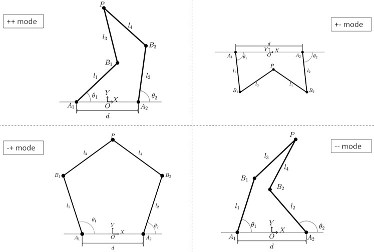
What is the meaning of “up‐configuration”? Based on the end-effector position within the reachable workspace, there are four possible working modes. A 5R planar robot arm typically has four different working modes. The notations “++, +-, -+, –” represent the four different possible configurations for working.

These modes arise from the different possible configurations of the robot’s links to reach a specific point in its workspace, which are related to the solutions of the inverse kinematics problem. Each mode represents a distinct way the robot can fold or extend its arm to achieve the desired position and orientation of its end-effector. The choice of working mode can affect the robot’s ability to avoid singularities and optimize its performance for specific tasks.

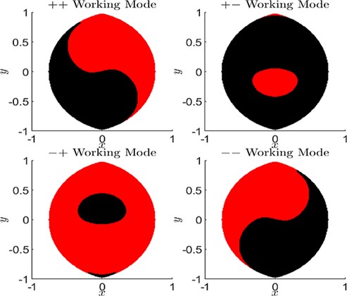
Our robot is using (-,+) mode. These signs refer to the angle of the joint. A₁ and A₂. Meaning how the angles are given to the motors. Here, angle A₁ will be -ve and angle A₂ will be +ve. This was just a simple overview, we will not go into detail for now.

6. Python Simulation of 5R Parallel Robot Arm

We can test our equations in Python. This Python code simulates the inverse kinematics of a 5-bar parallel robot and visualizes its motion along with an approximation of its reachable workspace. If a user gives any angle that is not reachable by the arm, it will show not reachable.

import sys
import math
import matplotlib.pyplot as plt
import numpy as np
import matplotlib.backend_bases

# Manipulator link lengths
l0 = 6.0    # Distance from the origin to left/right motor centers
l1 = 8.0    # Length from motor to passive joint
l2 = 8.0    # Length from passive joint to end effector

# Define the Y_MIN for the workspace calculation
Y_MIN = -15  # Adjust as needed

def calc_angles(x, y):
    # Angle from left shoulder to end effector
    beta1 = math.atan2( y, (l0 + x) )

    # Angle from right shoulder to end effector
    beta2 = math.atan2( y, (l0 - x) )

    # Alpha angle pre-calculations
    alpha1_calc = (l1**2 + ( (l0 + x)**2 + y**2 ) - l2**2) / (2*l1*math.sqrt( (l0 + x)**2 + y**2 ))
    alpha2_calc = (l1**2 + ( (l0 - x)**2 + y**2 ) - l2**2) / (2*l1*math.sqrt( (l0 - x)**2 + y**2 ))

    # If calculations > 1 or < -1, will fail acos function
    if alpha1_calc > 1 or alpha1_calc < -1 or alpha2_calc > 1 or alpha2_calc < -1:
        return None, None  # Indicate unreachable
    else:
        # Angle of left shoulder - beta1 and right shoulder - beta2
        alpha1 = math.acos(alpha1_calc)
        alpha2 = math.acos(alpha2_calc)

        # Angles of left and right shoulders
        shoulder1 = beta1 + alpha1
        shoulder2 = math.pi - beta2 - alpha2

        return(shoulder1, shoulder2)

def plot_arms(shoulder1, shoulder2, efx, efy):
    # Fixed points (motors)
    a1 = (-l0, 0)
    a2 = (l0, 0)

    # Passive joints (x, y) location
    p1 = ( -l0 + l1*math.cos(shoulder1), l1*math.sin(shoulder1)  )
    p2 = ( l0 + l1*math.cos(shoulder2), l1*math.sin(shoulder2)  )

    # End effector
    e = (efx, efy)

    # Unpack coordinates
    a1_x, a1_y = a1
    a2_x, a2_y = a2
    p1_x, p1_y = p1
    p2_x, p2_y = p2
    e_x, e_y = e

    # Left arm
    plt.plot([a1_x, p1_x, e_x], [a1_y, p1_y, e_y], 'bo-')
    plt.text(a1_x - 0.5, a1_y + 0.3, "A1")
    plt.text(p1_x + 0.3, p1_y + 0.3, "P1 ({:.2f}, {:.2f})".format(p1_x, p1_y), fontsize=8)
    plt.text(-l0+0.3, 0+0.3, "{:.2f} degrees".format(math.degrees(shoulder1)), fontsize=8)

    # Right arm
    plt.plot([a2_x, p2_x, e_x], [a2_y, p2_y, e_y], 'bo-')
    plt.text(a2_x + 0.3, a2_y + 0.3, "A2")
    plt.text(p2_x + 0.3, p2_y + 0.3, "P2 ({:.2f}, {:.2f})".format(p2_x, p2_y), fontsize=8)
    plt.text(l0+0.3, 0+0.3, "{:.2f} degrees".format(math.degrees(shoulder2)), fontsize=8)

    # EF
    plt.plot(e_x, e_y, 'ro')
    plt.text(e_x + 0.3, e_y + 0.3, "E ({:.2f}, {:.2f})".format(e_x, e_y), fontsize=8)

def on_press(event):
    if event.key == 'q':
        sys.exit()

def compute_workspace_boundary():
    """
    Computes a grid over the approximate workspace region and determines
    which (x, y) points are reachable by the robot.

    The robot is reachable at a point (x,y) if the distance between (x,y)
    and each motor (located at (-l0, 0) and (l0, 0)) is in the range:
        [|l1 - l2|, l1+l2].
    Returns:
        X, Y: Meshgrid arrays.
        reach: A 2D array with 1 for reachable and 0 for unreachable.
    """
    x_vals = np.linspace(-20, 20, 400)
    y_vals = np.linspace(Y_MIN, 20, 400)
    X, Y = np.meshgrid(x_vals, y_vals)
    r1 = np.sqrt((X + l0)**2 + Y**2)
    r2 = np.sqrt((l0 - X)**2 + Y**2)
    # Reachable condition for each chain
    cond1 = np.logical_and(r1 >= abs(l1 - l2), r1 <= (l1 + l2))
    cond2 = np.logical_and(r2 >= abs(l1 - l2), r2 <= (l1 + l2))
    reach = np.logical_and(cond1, cond2).astype(float)
    return X, Y, reach

def plot_plot(efx, efy, workspace_x, workspace_y, reach):
    plt.title('5-Bar Parallel Robot Kinematics')
    plt.contourf(workspace_x, workspace_y, reach, levels=[0.5, 1], colors=['lightgray'], alpha=0.5, label='Approximate Workspace')
    plt.plot(-20, -20, 'wo') # Invisible point to set lower bounds
    plt.plot(20, 20, 'wo')  # Invisible point to set upper bounds

    s1, s2 = calc_angles(efx, efy)
    if s1 is not None and s2 is not None:
        plot_arms(s1, s2, efx, efy)
        print(f"Coordinates Reachable: ({efx:.2f}, {efy:.2f})")
    else:
        plt.plot(efx, efy, 'rx', markersize=10, label='Unreachable') # Mark unreachable points

    plt.legend()
    plt.gca().set_aspect('equal', adjustable='box')
    plt.draw()
    plt.pause(0.1)
    plt.clf()

if __name__ == "__main__":
    fig = plt.figure()
    fig.canvas.mpl_connect('key_press_event', on_press)

    workspace_x, workspace_y, reach = compute_workspace_boundary()

    a1_x, a1_y = -l0, 0
    a2_x, a2_y = l0, 0

    while True:
        for i in range(-15, 16):
            plot_plot(i, 10, workspace_x, workspace_y, reach)
        for j in range(10, 16):
            plot_plot(15, j, workspace_x, workspace_y, reach)
        for k in range(15, -16, -1):
            plot_plot(k, 15, workspace_x, workspace_y, reach)
        for l in range(15, 9, -1):
            plot_plot(-15, l, workspace_x, workspace_y, reach)

Core Functionality:

1. Robot Definition: The code starts by defining the fixed link lengths of the robot: l0 (half the distance between the motor mounts), l1 (upper link length), and l2 (lower link length).
2. Inverse Kinematics (calc_angles(x, y)): This function takes the desired end effector coordinates (x, y) as input and calculates the required angles (shoulder1, shoulder2) of the two motor joints to reach that position. It uses geometric relationships and atan2 and acos functions. It also checks for unreachable coordinates (where a valid angle cannot be calculated).
3. Forward Kinematics (Implicit in Workspace Calculation): The compute_workspace_boundary() function implicitly uses forward kinematics concepts. It determines the reachable workspace by checking if a given point in space is at a valid distance from both motor mounts, considering the possible extensions and contractions of the individual arms (l1 + l2 down to |l1 - l2|).
4. Workspace Calculation (compute_workspace_boundary()): This function generates a grid of points and determines if each point is reachable by the robot. It does this by checking if the distance from each grid point to the two motor locations falls within the geometrically feasible range of the individual arms.
5. Visualization (plot_arms, plot_plot):
   • plot_arms() takes the calculated shoulder angles and end effector coordinates and draws the robot’s arms, passive joints (P1, P2), end effector (E), and motor mounts (A1, A2) on a Matplotlib plot. It also displays the joint angles and coordinates.
   • plot_plot() orchestrates the plotting process for each animation step. It plots the approximate workspace as a filled contour, and then, if the target end effector position is reachable, it draws the robot’s configuration. If the target is unreachable, it marks the point with a red ‘x’.
6. Animation Loop (if __name__ == "__main__":): The main part of the code sets up a Matplotlib figure and connects a key press event to allow the user to stop the animation by pressing ‘q’. It then enters an infinite loop that iterates through a predefined rectangular path of end effector coordinates. For each target coordinate, it calculates the required motor angles, plots the robot’s configuration (if reachable), and updates the display, creating the animation.
7. User Interaction: The program allows the user to stop the animation at any time by pressing the ‘q’ key while the plot window is active.

In essence, the code simulates the movement of a 5-bar parallel robot arm along a defined path while simultaneously visualizing the approximate area (workspace) that the end effector can reach based on the robot’s physical dimensions. The workspace is calculated by considering the reachability of points from each motor independently. The simulation highlights whether the robot can actually achieve the desired end effector positions within its kinematic constraints.

7. Limitations of the 5R Linkage Mechanism

It has a limited range of motion, and in some positions, it can run into tricky spots called singularities where control becomes difficult. But overall, its strengths make it a powerful tool in many areas of robotics. As cool and capable as the 5R robot arm is, it’s not perfect. There are a few important limitations to be aware of:

1. Limited Workspace
The area that the robot’s end-effector (the “hand” at the end of the arm) can reach isn’t as wide or flexible as that of a serial robot. Instead of being able to swing in large arcs or stretch out in different directions, the 5R arm is usually designed to operate within a specific flat area. Its reach depends a lot on the lengths of the links—if the link lengths are uneven, you can end up with awkward shapes or even “dead zones” in the workspace where the arm simply can’t go.

2. Singularity Issues
One tricky situation that can happen is called a singularity. This is a fancy way of saying the robot gets into a position where it starts to lose control over its motion. For example, if all the joints line up in a straight line, the arm might suddenly struggle to move in certain directions, kind of like when your arm is fully stretched out and you try to pull it straight back without bending it first. These spots are known trouble areas, and engineers work hard to avoid them when designing the robot’s movements.

3. Complex Math Behind the Scenes
If you want to tell the robot, “Move your hand to this exact point,” it has to figure out what angles each joint needs to be at—that’s called inverse kinematics. For 5R parallel robots, this calculation can get a bit messy compared to simpler serial arms. The good news? Most of this math is handled automatically by the robot’s control system, so users like you and me don’t have to sweat it too much.

8. References

1. Yang, T., Zhang, H., & Lee, W. (2018). “Analysis and Optimization of a 5R Planar Linkage Robot for High-Speed Pick-and-Place Operations”.
2. Sun, L., Wang, Q., & Chen, X. (2020). “Singularity Analysis and Avoidance Strategies for Planar 5R Linkage Systems”.
3. Louis Vathan. B, Hoshila Kumar, and Brighton Issac John .H. “Kinematic Analysis of Five-Bar Mechanism in Industrial Robotics”.
4. Mangesh D. Ratolikar1, Prasanth Kumar R. “Optimized design of 5R planar parallel mechanism aimed at gait-cycle of quadruped robots”.
5. Pentagon Robot, Five-bar robot Parallel SCARA linking to lead end-effector (SHOW1, side view)
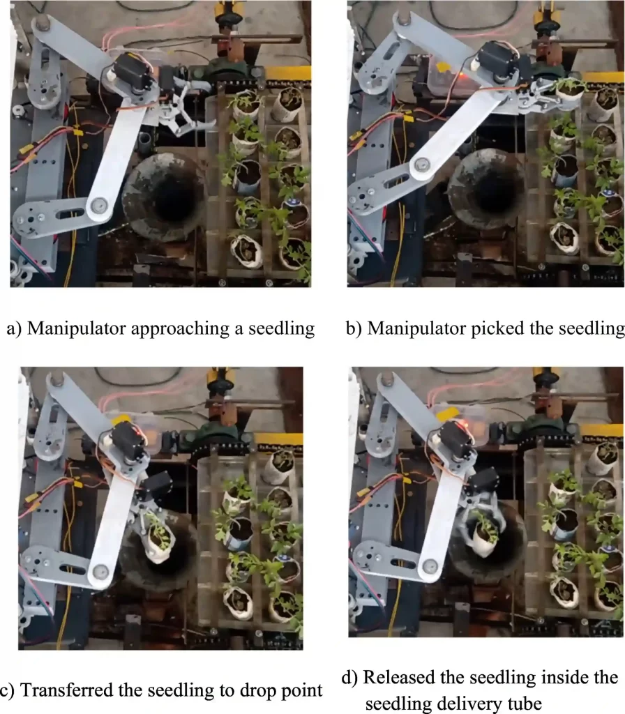
6. Design of a 4 DOF parallel robot arm and the firmware implementation on embedded system to transplant pot seedlings – ScienceDirect
7. GitHub – ddelago/5-Bar-Parallel-Robot-Kinematics-Simulation: Simulates the kinematics of a 5 bar planar manipulator using Python.